Introduction
Image classification is a fundamental task in computer vision with applications in medical imaging, autonomous driving, security, and e-commerce. As deep learning models advance, evaluating them correctly ensures reliability, minimizes errors, and enhances real-world performance.
Many data scientists rely on accuracy as the primary evaluation metric. However, accuracy can be misleading, especially when dealing with imbalanced datasets. To gain a more comprehensive understanding, we need to explore other metrics such as precision, recall, F1-score, confusion matrix, ROC curve, and AUC.
This guide explains these metrics, their significance, and best practices for optimizing model performance.
Why Accuracy Alone Is Not Enough
Understanding Accuracy
Accuracy provides an overall correctness measure:
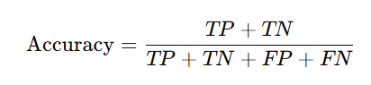
Where:
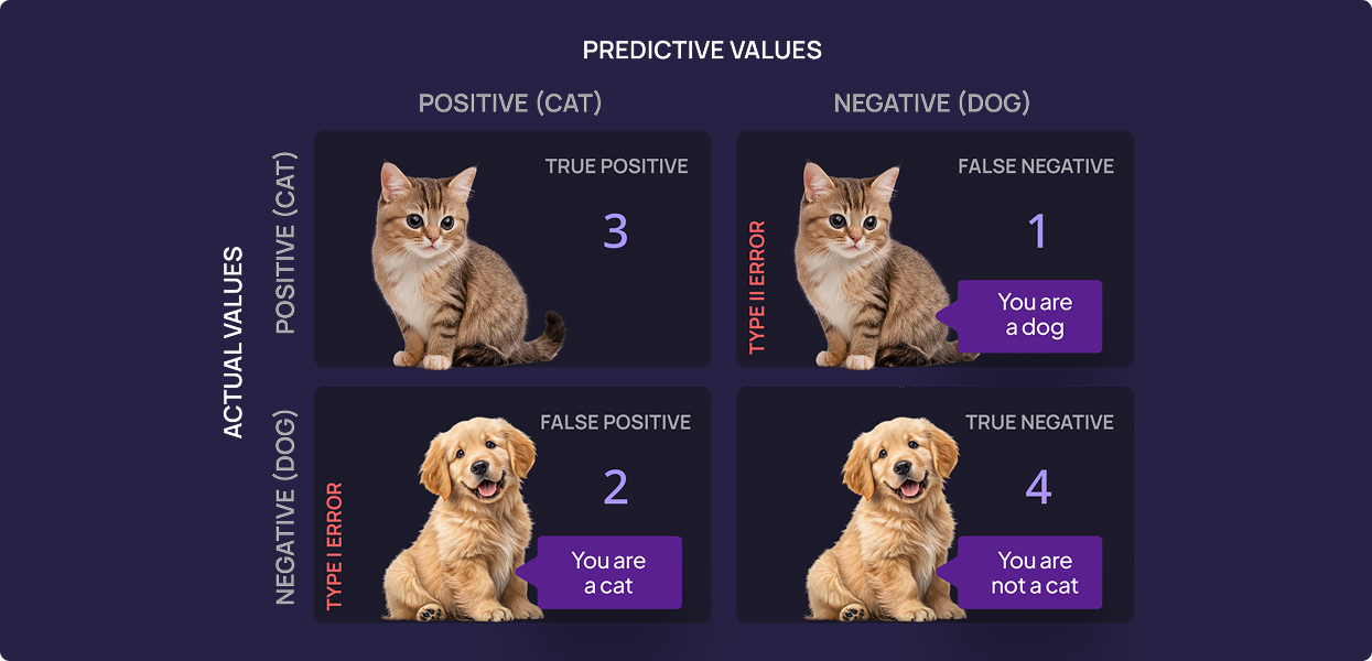
- True Positives (TP): Correctly classified positive images.
- True Negatives (TN): Correctly classified negative images.
- False Positives (FP): Negative images misclassified as positive.
- False Negatives (FN): Positive images misclassified as negative.
The Limitations of Accuracy
While easy to interpret, accuracy can be misleading. For instance, in a dataset where 95% of images belong to Class A and only 5% to Class B, a model that always predicts Class A achieves 95% accuracy but completely fails to recognize Class B.
This is particularly critical in applications like disease detection and fraud prevention, where detecting minority classes is crucial. Alternative metrics like precision, recall, and F1-score provide deeper insights.
Precision and Recall: The Essential Trade-Off
Precision
Precision measures how accurate the model’s positive predictions are:
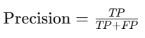
- High precision = fewer false positives.
- Useful when false positives have serious consequences.
Example: In fraud detection, a false positive could lead to blocking a legitimate transaction, causing inconvenience. High precision ensures only actual fraud cases are flagged.
Recall
Recall evaluates the model’s ability to correctly identify positive cases:
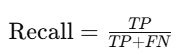
- High recall = fewer false negatives.
- Critical in scenarios like cancer detection and autonomous driving, where missing a positive case can be catastrophic.
Example: In autonomous vehicles, recall is crucial for pedestrian detection. Missing a pedestrian (false negative) could lead to serious accidents.
Precision vs. Recall: Finding the Right Balance
- High precision, low recall: The model is selective, reducing false positives but missing true positives.
- High recall, low precision: The model captures most positive cases but increases false positives.
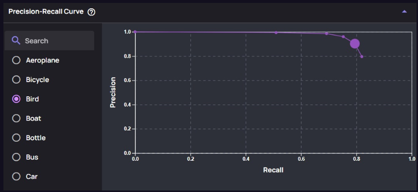
- The Precision-Recall Curve visualizes this trade-off and helps in selecting the optimal threshold.
Below is an example of a PR-Curve for the object “Bird,” showing how the curve’s shape is influenced by different threshold settings:
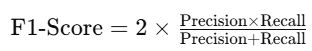
F1-Score: Combining Both Worlds
The F1-score balances precision and recall:
- Useful when false positives and false negatives are equally important.
- An F1-score close to 1 indicates a well-balanced model.
Example: In manufacturing defect detection, both false positives (discarding a good part) and false negatives (passing a faulty part) are problematic. The F1-score provides a way to balance the two requirements.
Confusion Matrix: A Detailed Error Analysis
A confusion matrix provides an in-depth breakdown of model predictions:
| Predicted Positive | Predicted Negative | |
| Actual Positive | True Positives (TP) | False Negatives (FN) |
| Actual Negative | False Positives (FP) | True Negatives (TN) |
- Helps identify misclassification patterns.
- Detects if the model is biased toward a particular class.
- Assists in adjusting classification thresholds.
ROC Curve and AUC: Evaluating Model Discrimination
ROC Curve – Receiver Operating Characteristic Curve
The ROC curve plots:
- True Positive Rate (TPR) = TP / (TP + FN)
- False Positive Rate (FPR) = FP / (FP + TN)
AUC – Area Under the Curve
The AUC measures the model’s ability to distinguish between classes:
- AUC = 1 → Perfect classifier.
- AUC > 0.9 → Excellent classifier.
- AUC = 0.5 → Random guessing.
AUC-ROC is widely used in medical diagnostics and fraud detection.
Additional Metrics
Log Loss – Logarithmic Loss
Log loss quantifies the uncertainty of predictions by penalizing incorrect predictions more heavily. It is defined as:

where:
- N is the total number of observations
- y_i is the actual class label (0 or 1)
- p_i is the predicted probability of the positive class
Lower log loss values indicate better performance.
Cohen’s Kappa
Measures agreement between predicted and actual labels, accounting for random chance.
- Used in medical diagnosis and sentiment analysis.
Matthews Correlation Coefficient (MCC)
The MCC is a balanced measure that takes into account all four confusion matrix categories (TP, TN, FP, FN). It is especially useful for imbalanced datasets and is calculated as:
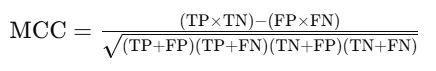
An MCC value of 1 indicates perfect prediction, 0 indicates no better than random chance, and -1 indicates total disagreement between actual and predicted values.
Akridata’s Model Evaluation
Akridata focuses on visual data and vision–related classifiers. Our Visual Copilot provides our users an interactive model evaluation system. It allows you to evaluate a model based on a confusion matrix, a PR–curve, F1 score per class and a way to see how each of those changes based on relevant thresholds.
Moreover, the above metrics are connected directly to the data, so when a misprediction is identified, you can see the ground truth labels and model predictions and make an informed decision as to how to improve the model’s quality the next training cycle.
Conclusion
Evaluating an image classification model requires more than just accuracy. By using precision, recall, F1-score, confusion matrices, and AUC-ROC, you gain deeper insights into model performance.
Akridata Visual Copilot provides an interactive way to see how a model performs based on the above mentioned metrics and supports you in improving the model during the next training cycle.


No Responses